Cilkscale — scalability analysis & benchmarking tool

users guide cilkscale tools

Cilkscale can help you reason about the parallel performance and scalability of your Cilk program. Cilkscale enables you to:

Collect statistics of parallel performance for your application.
Measure the work, span, and parallelism of your (sub-)computations and predict how their performance will scale on multiple processors.
Automatically benchmark your program on different numbers of processors.
Produce tables and graphical plots with the above performance and scalability measurements.

This guide will walk you through the basic steps of profiling the parallel performance and scalability of your Cilk application with Cilkscale. By the end of this guide, you will know how to generate performance and scalability tables and plots like the ones shown below and have a basic understanding of how to use them to diagnose parallel performance limitations of your application. For details on the Cilkscale components, user options, and output information, see the Cilkscale reference page.

Note:

This guide assumes that OpenCilk is installed within /opt/opencilk/ and that the OpenCilk C++ compiler can be invoked from the terminal as /opt/opencilk/bin/clang++, as shown in this example.

System setup for reported performance measurements:

All timings reported in this page are measured on a laptop with an 8-core Intel Core i7-10875H CPU, using OpenCilk 2.0.1 on Ubuntu 20.04 (via the Windows Subsystem for Linux v2 on Windows 10).

Example application

We shall illustrate how to use the various components of Cilkscale with a Cilk/C++ application that implements a parallel divide-and-conquer quicksort. The source code for our simple program, qsort.cpp, is shown below.

#include <iostream>
#include <algorithm>
#include <random>
#include <cilk/cilk.h>

constexpr std::ptrdiff_t BASE_CASE_LENGTH = 32;

template <typename T>
void sample_qsort(T* begin, T* end) {
  if (end - begin < BASE_CASE_LENGTH) {
    std::sort(begin, end);  // base case: serial sort
  } else {
    --end;  // exclude last element (pivot) from partition
    T* middle = std::partition(begin, end,
                               [pivot=*end](T a) { return a < pivot; });
    std::swap(*end, *middle);  // move pivot to middle
    cilk_scope {
      cilk_spawn sample_qsort(begin, middle);
      sample_qsort(++middle, ++end);  // exclude pivot and restore end
    }
  }
}

int main(int argc, char* argv[]) {
  long n = 100 * 1000 * 1000;
  if (argc == 2)
    n = std::atoi(argv[1]);

  std::default_random_engine rng;
  std::uniform_int_distribution<long> dist(0,n);
  std::vector<long> a(n);
  std::generate(a.begin(), a.end(), [&]() { return dist(rng); });

  std::cout << "Sorting " << n << " random integers" << std::endl;
  sample_qsort(a.data(), a.data() + a.size());

  bool pass = std::is_sorted(a.cbegin(), a.cend());
  std::cout << "Sort " << ((pass) ? "succeeded" : "failed") << "\n";
  return (pass) ? 0 : 1;
}

The qsort.cpp program simply generates a vector of pseudorandom numbers, sorts it in parallel with the sample_qsort() function, and verifies the result. We can compile and run it as follows.

$ /opt/opencilk/bin/clang++ qsort.cpp -fopencilk -O3 -o qsort
$ ./qsort 100000000
Sorting 100000000 random integers
Sort succeeded

Benchmarking and work/span analysis

Cilkscale instruments your Cilk program to collect performance measurements during its execution. Cilkscale instrumentation operates in one of two modes:

Benchmarking mode: Cilkscale measures the wall-clock execution time of your program.
Work/span analysis mode: Cilkscale measures the work, span, and parallelism of your program.

In either mode, you can use Cilkscale with two simple steps:

Pass a Cilkscale instrumentation flag to the OpenCilk compiler when you compile and link your program. The result is a Cilkscale-instrumented binary.
Run the instrumented binary. Cilkscale collects performance measurements and prints them to the standard output. (To output the report to a file, set the CILKSCALE_OUT environment variable.) Your program otherwise runs as it normally would.

By default, Cilkscale only reports performance results for whole-program execution. We will see how to perform fine-grained analyses of specific sub-computations in the next section, after we show how to use Cilkscale in benchmarking and work/span analysis mode.

Benchmarking instrumentation

To benchmark your application with Cilkscale, pass the -fcilktool=cilkscale-benchmark flag to the OpenCilk compiler:

$ /opt/opencilk/bin/clang++ qsort.cpp -fopencilk -fcilktool=cilkscale-benchmark -O3 -o qsort_cs_bench

Running the instrumented binary now produces the program output as before, followed by two lines with timing results in CSV format:

$ ./qsort_cs_bench 100000000
[...]
tag,time (seconds)
,2.29345

The report table above contains a single, untagged row with the execution time for the entire program. We will see shortly that if we use the Cilkscale API for fine-grained analysis, then the report table will contain additional rows.

Work/span analysis instrumentation

To analyze the parallel scalability of your application with Cilkscale, pass the -fcilktool=cilkscale flag to the OpenCilk compiler:

$ /opt/opencilk/bin/clang++ qsort.cpp -fopencilk -fcilktool=cilkscale -O3 -o qsort_cs

When you run the instrumented binary, the program output is followed by the Cilkscale work/span analysis report in CSV format:

$ ./qsort_cs 100000000
[...]
tag,work (seconds),span (seconds),parallelism,burdened_span (seconds),burdened_parallelism
,26.9397,2.29954,11.7153,2.29986,11.7136

The work, span, and parallelism measurements in the report depend on your program's input and logical parallelism but not on the number of processors on which it is run. The Cilkscale reference page describes the specific quantities reported by Cilkscale.

As before, the reported measurements above are untagged and refer to whole-program execution.

Note:

The Cilkscale-instrumented binary in work/span analysis mode is slower than its non-instrumented counterpart. The slowdown is generally no larger than 10x and typically less than 2x. In the examples above, qsort and qsort_cs_bench took 2.3s while qsort_cs took 3.4s (slowdown = 1.5x).

Fine-grained analysis

Cilkscale provides a C/C++ API for benchmarking or analyzing specific regions in a program. The Cilkscale API allows you to focus on and distinguish between specific parallel regions of your computation when measuring its parallel performance and scalability. Using the Cilkscale API is similar to using common C/C++ APIs for timing regions of interest (such as the C++ std::chrono library or the POSIX clock_gettime() function).

Let's see how we can use the Cilkscale API to analyze the execution of sample_qsort() function in our example quicksort application. That is, we want to exclude the computations for initializing a random vector of integers or verifying the sort correctness, which are all executed serially anyway. To achieve this, make the following three changes to the code.

Include the Cilkscale API header file. E.g., after line 4 in qsort.cpp:
```
#include <cilk/cilkscale.h>
```
Create work-span snapshots using calls to wsp_getworkspan() around the region we want to analyze. E.g., around the call to sample_qsort() in line 35 in qsort.cpp:
```
wsp_t start = wsp_getworkspan();
sample_qsort(a.data(), a.data() + a.size());
wsp_t end = wsp_getworkspan();
```
Evaluate the work and span between the relevant snapshots and print the analysis results with a descriptive tag. E.g., just before the program terminates in line 39 in qsort.cpp:
```
wsp_t elapsed = wsp_sub(end, start);
wsp_dump(elapsed, "qsort_sample");
```

Then, save the edited program (here, we save it as qsort_wsp.cpp), compile it with Cilkscale instrumentation as before, and run it:

$ /opt/opencilk/bin/clang++ qsort_wsp.cpp -fopencilk -fcilktool=cilkscale -O3 -o qsort_wsp_cs
$ ./qsort_wsp_cs 100000000
[...]
tag,work (seconds),span (seconds),parallelism,burdened_span (seconds),burdened_parallelism
sample_qsort,26.1502,1.08122,24.1859,1.08153,24.1788
,27.3133,2.24433,12.1699,2.24465,12.1682

Notice that the Cilkscale report above now contains an additional row tagged sample_qsort, which was output by the corresponding call to wsp_dump():

sample_qsort,26.1502,1.08122,24.1859,1.08153,24.1788

The last row in the Cilkscale report is always untagged and corresponds to the execution of the whole program.

Note:

If you compile your code without a Cilkscale instrumentation flag, calls to the Cilkscale API are effectively ignored with zero overhead.

For more detailed information on the Cilkscale C/C++ API, as well as an example of how to aggregate work/span analysis measurements from disjoint code regions, see the relevant section of the Cilkscale reference page.

Automatic scalability benchmarks and visualization

Cilkscale includes a Python script which automates the process of benchmarking and analyzing the scalability of your Cilk program. Specifically, the Cilkscale Python script helps you do the following:

Collect work/span analysis measurements for your program.
Benchmark your program on different numbers of processors and collect empirical scalability measurements.
Store the combined analysis and benchmarking results in a CSV table.
Visualize the analysis and benchmarking results with informative execution time and speedup plots.

The Cilkscale Python script is found at share/Cilkscale_vis/cilkscale.py within the OpenCilk installation directory.

Prerequisites:

To use the Cilkscale Python script, you need:

Python 3.8 or later.
(Optional) matplotlib 3.5.0 or later; only required if producing graphical plots.

How to run

To use the cilkscale.py script, you must pass it two Cilkscale-instrumented binaries of your program — one with -fcilktool=cilkscale-benchmark and one with -fcilktool=cilkscale — along with a number of optional arguments. For a description of the cilkscale.py script's arguments, see the Cilkscale reference page.

Let's now see an example of using the cilkscale.py script to analyze and benchmark our qsort_wsp.cpp program, which uses the Cilkscale API to profile the sample_qsort() function. First, we build the two Cilkscale-instrumented binaries:

$ /opt/opencilk/bin/clang++ qsort_wsp.cpp -fopencilk -fcilktool=cilkscale-benchmark -O3 -o qsort_cs_bench
$ /opt/opencilk/bin/clang++ qsort_wsp.cpp -fopencilk -fcilktool=cilkscale -O3 -o qsort_cs

Then, we run cilkscale.py with our instrumented binaries on a sequence of 100,000,000 random integeres, and specify the output paths for the resulting CSV table and PDF document of visualization plots:

$ python3 /opt/opencilk/share/Cilkscale_vis/cilkscale.py \
    -c ./qsort_cs -b ./qsort_cs_bench \
    -ocsv cstable_qsort.csv -oplot csplots_qsort.pdf \
    --args 100000000

Terminal output

The cilkscale.py script first echoes the values for all of its parameters, including unspecified parameters with default values:

Namespace(args=['100000000'], cilkscale='./qsort_cs', cilkscale_benchmark='./qsort_cs_bench', cpu_counts=None, output_csv='cstable_qsort.csv', output_plot='csplots_qsort.pdf', rows_to_plot='all')

Then, it runs the instrumented binary for work/span analysis on all available cores and prints its standard output and standard error streams. You should make sure that the program output is as expected.

>> STDOUT (./qsort_cs 100000000)
Sorting 100000000 random integers
Sort succeeded
<< END STDOUT

>> STDERR (./qsort_cs 100000000)
<< END STDERR

Once the work/span analysis pass is done, cilkscale.py runs the instrumented binary for benchmarking on different numbers of processors. The number of benchmarking runs and corresponding numbers of processors are determined by the -cpus arguments to cilkcsale.py. (If this argument is not specified, the program will run on $1, 2, \dots, P$ processors, where $P$ is the number of available physical cores in the system.)

INFO:runner:Generating scalability data for 8 cpus.
INFO:runner:CILK_NWORKERS=1 taskset -c 0 ./qsort_cs_bench 100000000
INFO:runner:CILK_NWORKERS=2 taskset -c 0,2 ./qsort_cs_bench 100000000
INFO:runner:CILK_NWORKERS=3 taskset -c 0,2,4 ./qsort_cs_bench 100000000
INFO:runner:CILK_NWORKERS=4 taskset -c 0,2,4,6 ./qsort_cs_bench 100000000
INFO:runner:CILK_NWORKERS=5 taskset -c 0,2,4,6,8 ./qsort_cs_bench 100000000
INFO:runner:CILK_NWORKERS=6 taskset -c 0,2,4,6,8,10 ./qsort_cs_bench 100000000
INFO:runner:CILK_NWORKERS=7 taskset -c 0,2,4,6,8,10,12 ./qsort_cs_bench 100000000
INFO:runner:CILK_NWORKERS=8 taskset -c 0,2,4,6,8,10,12,14 ./qsort_cs_bench 100000000

In this example, the program is benchmarked on up to 8 CPU cores with IDs 0, 2, 4, …. This is because cilkscale.py only uses distinct physical cores by default. In the computer used for this example, core IDs 1, 3, 5, … correspond to logical cores used in simultaneous multithreading or "hyper-threading".

Finally, cilkscale.py processes the collected benchmarking and work/span analysis measurements and generates runtime and speedup plots for each analyzed region (and the entire program).

INFO:plotter:Generating plot (2 subplots)

The Cilkscale benchmarking and scalability analysis reports are returned in tabular and graphical form.

Tabular output

The raw measurements are output as a CSV table in the file pointed to by the -ocsv argument to cilkscale.py. The CSV table contains, for each analyzed region, the work/span analysis results and benchmark times for all numbers of processors.

For example, the above run produced the following table:

$ cat cstable_qsort.csv
tag,work (seconds),span (seconds),parallelism,burdened_span (seconds),burdened_parallelism,1c time (seconds),2c time (seconds),3c time (seconds),4c time (seconds),5c time (seconds),6c time (seconds),7c time (seconds),8c time (seconds)
sample_qsort,26.5126,0.986602,26.8726,0.986927,26.8638,8.67705,4.6205,3.3648,2.75881,2.43091,2.1171,1.93193,1.7941
,27.6918,2.16583,12.7858,2.16616,12.7839,9.68071,5.52596,4.26341,3.65358,3.32762,3.02633,2.82155,2.67563

To see the table contents more clearly, you can import cstable_qsort.csv into a spreadsheet (e.g., with LibreOffice) or pretty-print it with command-line tools:

$ cat cstable_qsort.csv | sed -e 's/^,/ ,/g' | column -s, -t | less -#5 -N -S
1 tag           work (seconds)  span (seconds)  parallelism  burdened_span (seconds)  burdened_parallelism 1c time (seconds)  . . .
2 sample_qsort  26.5126         0.986602        26.8726      0.986927                 26.8638              8.67705             . . .
3               27.6918         2.16583         12.7858      2.16616                  12.7839              9.68071            . . .

Scalability plots

Cilkscale produces a set of scalability plots from the raw measurements in its reported table. These plots are stored the PDF file pointed to by the -oplot argument to cilkscale.py. Specifically, Cilkscale produces two figures for each analyzed region (i.e., row in the CSV table): one which plots execution time and one which plots parallel speedup. For a more detailed description of these plots' contents, see the Cilkscale reference page.

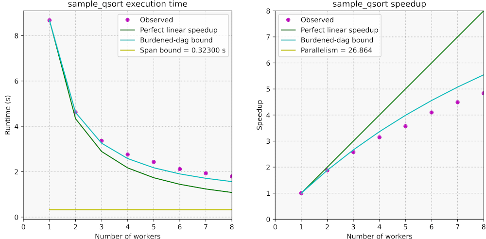
Here are the plots in csplots_qsort.pdf for the above example:

Discussion: diagnosing performance limitations

We have seen how to measure and explore the parallel performance and scalability of a Cilk program. So... what next? How can we translate the Cilkscale results into actionable insights on how to improve performance? As with serial-program profiling, the answer varies somewhat depending on the program at hand. We will return to this question with forthcoming documentation and blog posts. Please let us know if you'd like to be notified about important updates to OpenCilk and its documentation.

In the meantime, we offer a brief discussion regarding the parallel scalability of our qsort.cpp example, specifically the sample_qsort() function.

We observe the following:

Our program shows sub-linear scalability. With 8 processor cores, the parallel speedup is only about 4.9x.
The observed performance roughly follows the burdened-dag bound and falls short of it as the number of cores increases.
The parallelism of sample_qsort() is about 27, which is just over three times as large as the amount of cores on the laptop where the experiments were run.

A main issue with our parallel sample_qsort() is that it does not exhibit sufficient parallelism. The parallelism of a computation upper-bounds the number of processors that may productively work in parallel. Moreover, computations with insufficient parallel slackness are typically impacted adversely by scheduling and migration overheads. As a rule of thumb, the parallelism of a computation is deemed sufficient if it is about 10x larger (or more) than the number of available processors. On the other hand, if the parallelism is too high — say, several orders of magnitude higher than the number of processors — then the overhead for spawning tasks that are too fine-grained may become substantial. In our case, the parallelism is low and exhibits sufficient slackness for only 2–3 cores.

An additional issue is that the memory bandwidth of the laptop that was used in these experiments becomes insufficient as more processing cores are used. This is often the case for computations with low arithmetic intensity when the observed parallel speedup falls below the burdened-dag speedup bound. (Another possible cause for speedup below the burdened-dag bound is contention of parallel resources.) The memory bandwidth ceiling was measured at about 24 GB/s with the STREAM "copy" benchmark in either serial or parallel mode.

If we want to improve the parallel performance of sample_qsort(), it appears that our efforts, at least initially, are best spent increasing its parallelism. One way to do that might be to undo the coarsening of the base case (e.g., setting BASE_CASE_LENGTH = 1) but that makes the recursion too fine-grained and introduces unnecessary spawning overhead — that is, we may get better parallel speedup but slower execution overall. The one remaining option then is to parallelize std::partition(), which is currently serial and whose cost is linear with respect to the size of the input array.

We will not cover parallel partition algorithms for quicksort here, but warn that designing and implementing efficient parallel partitions is an interesting and nontrivial exercise!

On this page

Cilkscale — scalability analysis & benchmarking tool

Example application #

Benchmarking and work/span analysis #

Benchmarking instrumentation #

Work/span analysis instrumentation #

Fine-grained analysis #

Automatic scalability benchmarks and visualization #

How to run #

Terminal output #

Tabular output #

Scalability plots #

Discussion: diagnosing performance limitations #

Example application

Benchmarking and work/span analysis

Benchmarking instrumentation

Work/span analysis instrumentation

Fine-grained analysis

Automatic scalability benchmarks and visualization

How to run

Terminal output

Tabular output

Scalability plots

Discussion: diagnosing performance limitations